The machining module has two machines integrated in one model, the CNC and admission module.
The CNC machine was designed by Julian Luna and Alejandro Ojeda for the Sensors and Actuators class at UNAL. You can view the design document in the following link.
CNC
- The machine has a 50 cm x 25 cm work area.
- The machine mills using a Dremel 4000 and a 30° V type milling bit.
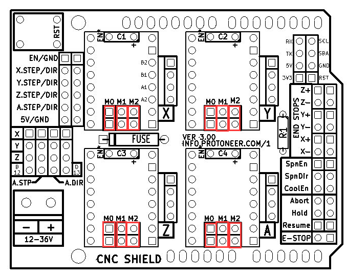
- The machine controller uses an Arduino UNO and a CNC shield board. The firmware running is GRBL.
Mechanical Design
Torque Calculation
The calculation of torque is carried out based on the torque equation for lifting a piece according to Shigley. \cite{shigley1985mechanical}
\[T_R=\frac{F d_m}{2} (\frac{l + f \pi d_m}{\pi d_m - f l})\]Where:
\(T_R\) is the required torque. \(d_m\) is the mean diameter, or \(d_m = d - 0.5p\), where \(d\) is the outer diameter and \(p\) the pitch \(f\) is the friction coeficient \(l\) is the lead \(F\) is the axial force
And reordering the equation it was obtained that
\[\frac{2 T_R}{d_m} (\frac{ \pi d_m - f l} {l + f \pi d_m}) = F\]The obtained force for the machine is \(T_R=0.308 \, Nm\)
Angle Brackets
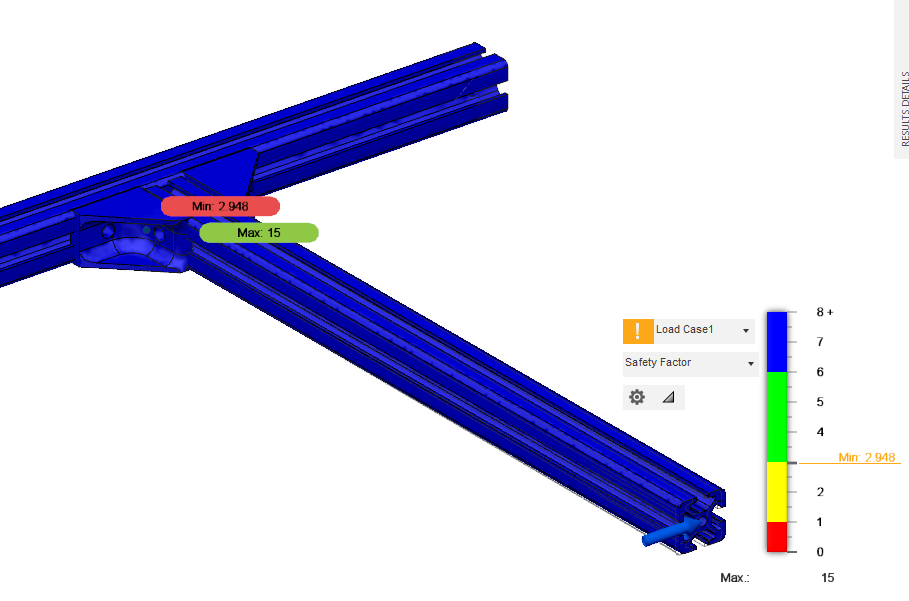
Angle brackets were designed to support the base structure forces, all the aluminium profiles connect the ends where angle brackets provide support. Due to the load they willl support during the machine operation, forces over the bracket were analyzed, to provide a Factor of Safety (FoS) on the design. The tool used to analyze the FoS was finite element simluation in Autodesk Fusion 360. The force over the bracket is calculated as follows:
\(T_R=0.014 \, Nm\) \(d_m=0.007 \, m\) The coeficient between steel and bronze: \(f=0.15\)
\(l=0.008 \,m\) \(F=(\frac{2 T_R}{d_m}) (\frac{\pi d_m - fl}{l + f\pi d_m})=7.636 \,N\)
In the scenario where only one bracket is tightened correctly the following figure shows the FoS at the end of the aluminium profile. In this case is \(2.948\).
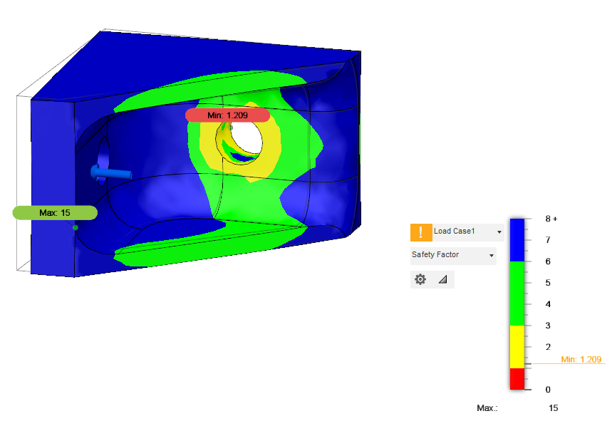
For the bracket itself (in the same scenario) the response is shown in the following figure, with a value of \(1.209\).
FoS on the Angle bracket for the worst case scenario.
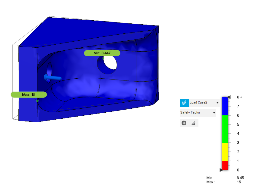
In the general case, the structure will count with two brackets, each with 4 fasteners, so the model obtained for this is shown in the next figure, where the minimal FoS is \(8.45\).
FoS on the Angle bracket in its standard functioning
Additive Manufacturing
All the printed parts were manufactured in the FDM printer ar the LabFabEx. White PLA by 3DBots was used, with \(0.8\,mm\) walls, \(70\%\) cubic infill, raft support and a \(50\,mm\) printing speed.
Axis support printing
X axis support fit in the aluminium profile
Motor, support and base corner fit.
Geometric Dimensioning and Tolerancing
In order to verify the manufacturing process multiple tolerancing methods were monitored and executed.
In order to verify the tolerance of the 3D FDM Printer at the laboratory, a test tool to validate the tolerance was designed and printed. The model is shown in figure next figure.
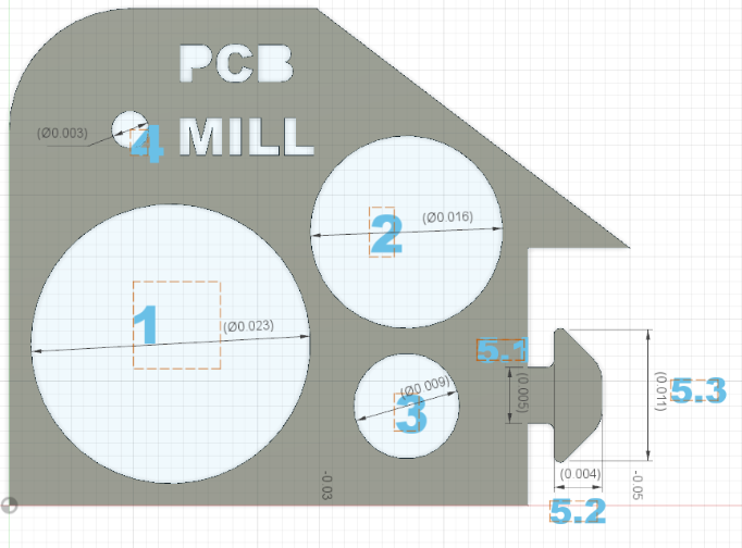
Printing tolerance validation piece.
The measurements were registered in the table ahead, and the error was calculated in it. Measurements were taken using a caliper.
| Reference | Measurement No | Value | Mean Value | Error value | Absolute Error | Nominal Value | Value with tolerance | Relative error |
|---|---|---|---|---|---|---|---|---|
| 1 | 1 | 22,10 | 22,13 | 0,12 | 0,37 | 23,00 | 22,50 | 0,25 |
| ~ | 2 | 22,08 | ~ | ~ | ~ | ~ | ~ | ~ |
| ~ | 3 | 22,20 | ~ | ~ | ~ | ~ | ~ | ~ |
| 2 | 1 | 15,12 | 15,18 | 0,14 | 0,32 | 16,00 | 15,50 | 0,18 |
| ~ | 2 | 15,16 | ~ | ~ | ~ | ~ | ~ | ~ |
| ~ | 3 | 15,26 | ~ | ~ | ~ | ~ | ~ | ~ |
| 3 | 1 | 8,12 | 8,13 | 0,16 | 0,37 | 9,00 | 8,50 | 0,21 |
| ~ | 2 | 8,06 | ~ | ~ | ~ | ~ | ~ | ~ |
| ~ | 3 | 8,22 | ~ | ~ | ~ | ~ | ~ | ~ |
| 4 | 1 | 2,60 | 2,64 | 0,10 | -0,14 | 3,00 | 2,50 | -0,24 |
| ~ | 2 | 2,62 | ~ | ~ | ~ | ~ | ~ | ~ |
| ~ | 3 | 2,70 | ~ | ~ | ~ | ~ | ~ | ~ |
| 5.1 | 1 | 5,06 | 4,99 | 0,34 | 0,51 | 5,00 | 5,50 | 0,17 |
| ~ | 2 | 4,78 | ~ | ~ | ~ | ~ | ~ | ~ |
| ~ | 3 | 5,12 | ~ | ~ | ~ | ~ | ~ | ~ |
| 5.2 | 1 | 4,20 | 4,40 | 0,76 | 0,10 | 4,00 | 4,50 | -0,66 |
| ~ | 2 | 4,12 | ~ | ~ | ~ | ~ | ~ | ~ |
| ~ | 3 | 4,88 | ~ | ~ | ~ | ~ | ~ | ~ |
| 5.3 | 1 | 11,08 | 11,69 | 0,92 | -0,41 | 10,78 | 11,28 | -1,33 |
| ~ | 2 | 12,00 | ~ | ~ | ~ | ~ | ~ | ~ |
| ~ | 3 | 11,98 | ~ | ~ | ~ | ~ | ~ | ~ |
| 5.4 | 1 | 1,84 | 1,83 | 0,06 | -0,33 | 2,00 | 1,50 | -0,39 |
| ~ | 2 | 1,86 | ~ | ~ | ~ | ~ | ~ | ~ |
Small holes were also measured using the Zoller machine at the laboratory. The error perceived for the reference \(1\) was \(1.0740\,mm\), for reference \(4\) is \(0.088\,mm\), for reference \(5.1\) is \(0.037\,mm\) and for reference \(5.4\) is \(0.019\,mm\).
Errors found in the measurements are shown in graph the next graph.
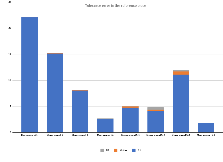
Tolerance error in the reference piece.
After knowing the tolerances for the machine production quality, and given that multiple Commercial Off The Shelve parts were selected, a Shaft-based system was selected.
For clearance fit, parts should be able to move slightly.
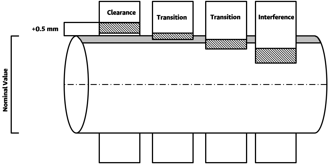 Clearance Fit.
Transition fit tries to make objects are firm but not under pressure, making it easy to remove.
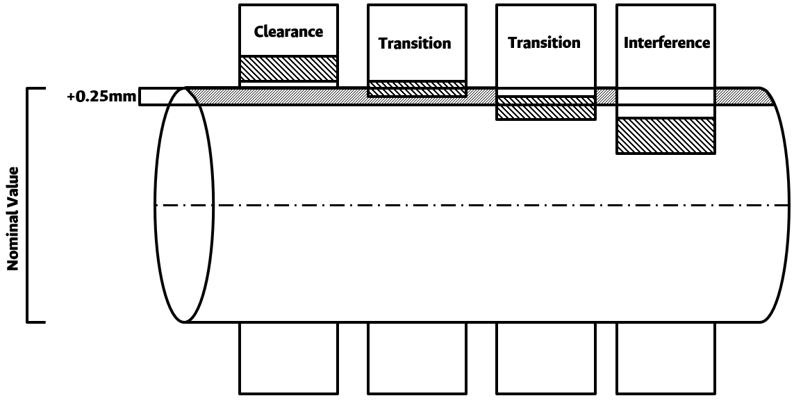 Transition Fit.
Interference fit is used to use pressure to place an element on another, typically to be fixed permanently.
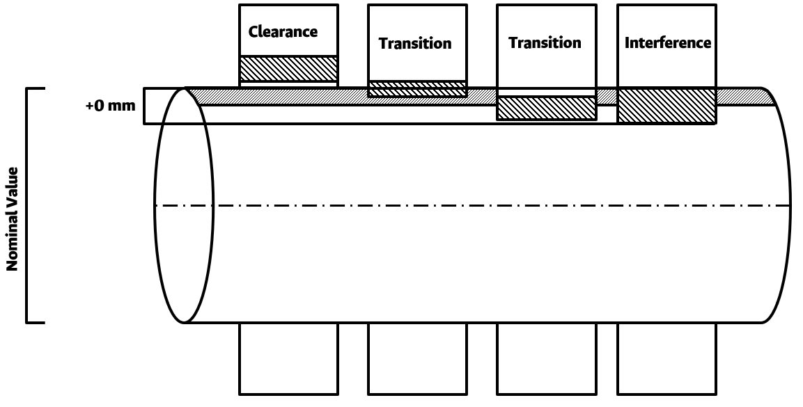 Interference Fit.
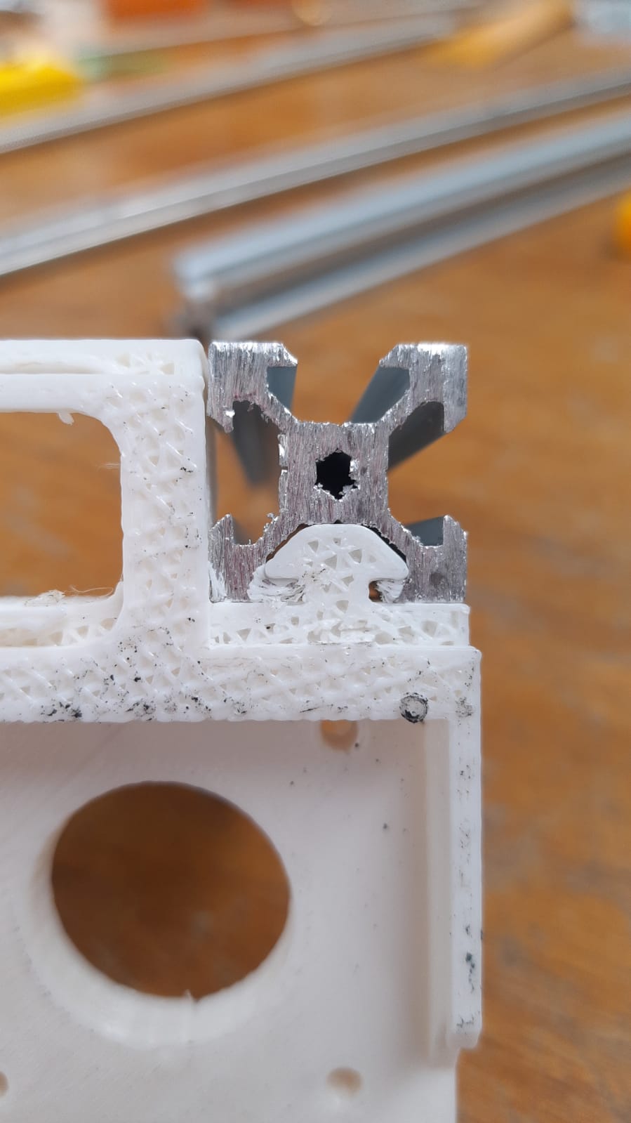
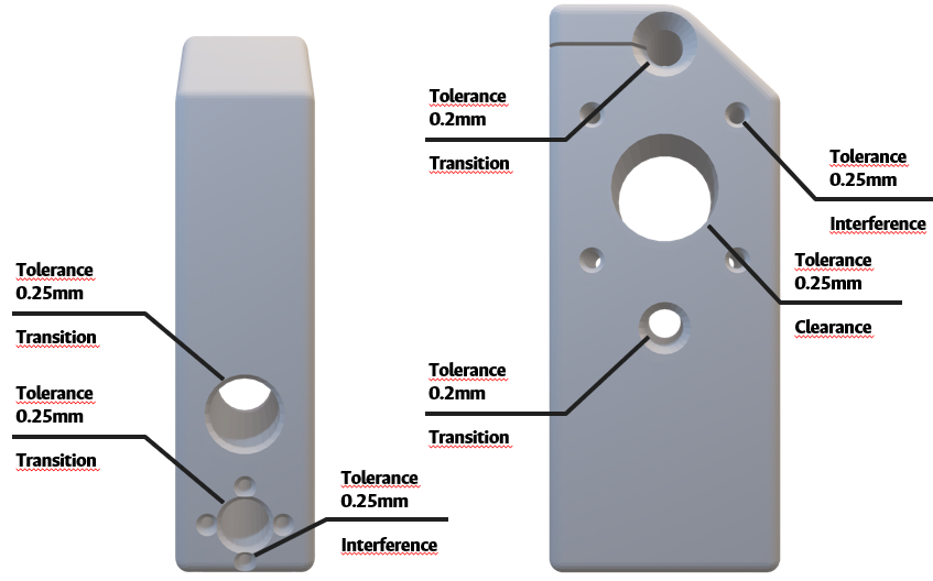
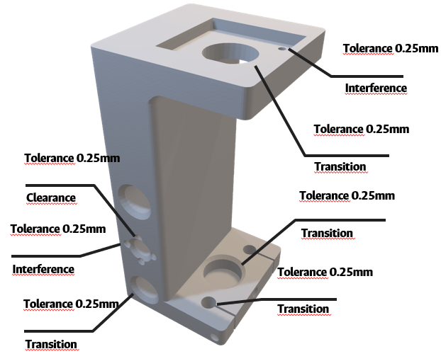
Every element that was manufactured using Additive Manufacturing defined the type of fit that was required. For the X axis support it’s elements fit are shown in figure gdt1. Y axis supports are shown in figure gdt2.
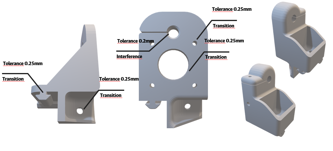
Fit for X axis supports.
Y axis supports fit.
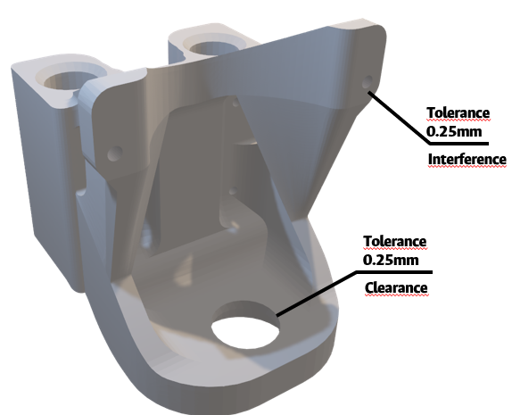
For the Dremel carriage two parts are defined, the Z axis support and the Dremel carraige itself. The first one is shown in figure gdt3, and the second one in figure gdt4 and gdt5.
Z axis support fit.
Fit for Dremel carriage (Front).
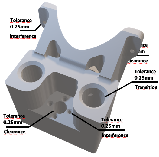
Fit for Dremel carriage (Back).
For the assembly process the following aspects of geometric control were used:
- Shape
- Straightness
- Flatness
- Orientation
- Parallelism
- Perpendicularity
- Angularity
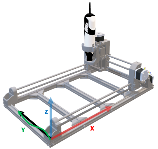
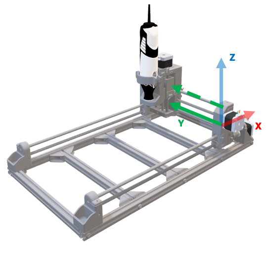
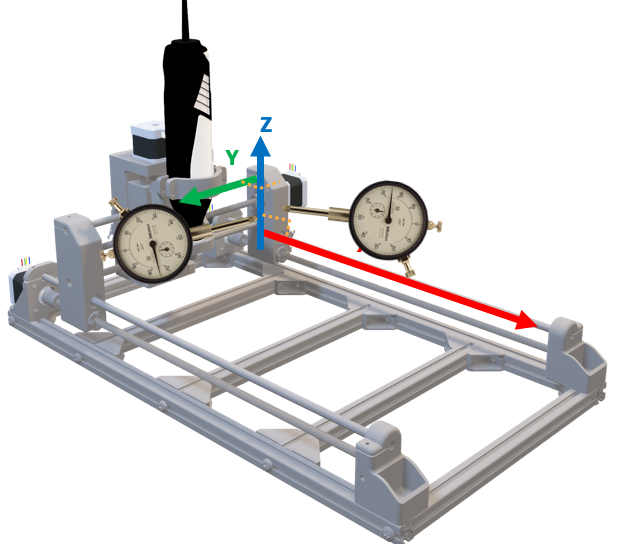
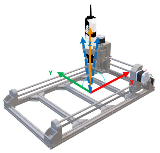
The following coordinate axis was used as reference, shown in figure gdyt1
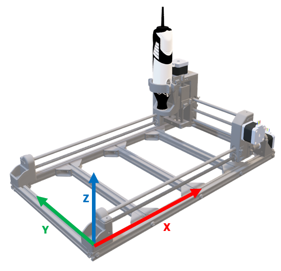
Coordinate axis.
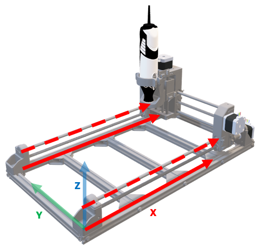
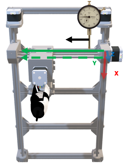
First straightness was checked for the X axis gdyt2, using a dial gauge on the surface gdyt3 and the Y axis gdyt4.
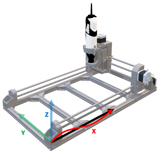
Straightness of X axis.
Usage of the dial gauge.
Straightness of the Y axis.
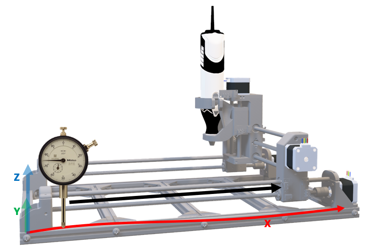
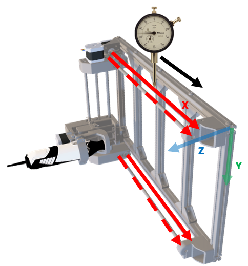
Parallellism was checked between the axis rod and the leadscrew gdyt5 using the method shown in figure gdyt6. As well as one Y axis gdyt7 using the method in figure gdyt8.
Aluminium profile cuts for each phase.
Aluminium profile cuts for each phase.
Aluminium profile cuts for each phase.
Aluminium profile cuts for each phase. Perpendicularity was verified between the X and Y axis gdyt9.
Aluminium profile cuts for each phase.
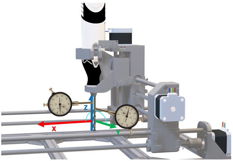
Finally, angularity was studied between the Z axis vs the XY plane gdyt10 using the method shown in figure gdyt11.
Aluminium profile cuts for each phase.
Aluminium profile cuts for each phase.
Manufacturing
Two types of profiles were used, a long one for the x-axis base, and 5 profiles placed perpendicularly to the x-axis, placed evenly. Due to the use of sliding printed supports, there was no need to have eaxct measurements, but the other profiles needed as much, because a different size meant irregularity in the paralellism. For this reason, they were selected in two groups, one for the ends and another for the interior ones.
To cut the profiles, first a hand saw was used, then a file was used to improve the regularity, and to obtain the final value the Leadwell CNC Machine at LabFabEx was used to mill the ends. In figure profilecut the three phases are shown. In the left, the profile was cut with the handsaw, in the middle it was filed and the final one was after being milled. The ones used at the end were threaded using an M5 tap. A \(\frac{5}{32} \, inch\) was tested, but it was too loose to be used.
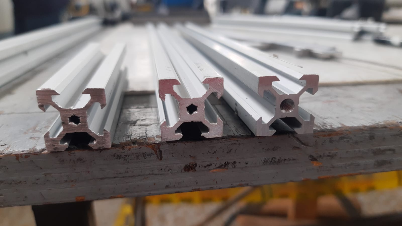
Aluminium profile cuts for each phase.
The milling process is shown in figure manufactura1. The mounting of the aluminium profile on the machine is shown in figure manufactura14, where a dial gauge was placed on the Leadwell’s head to verify every profile was placed in the same position.
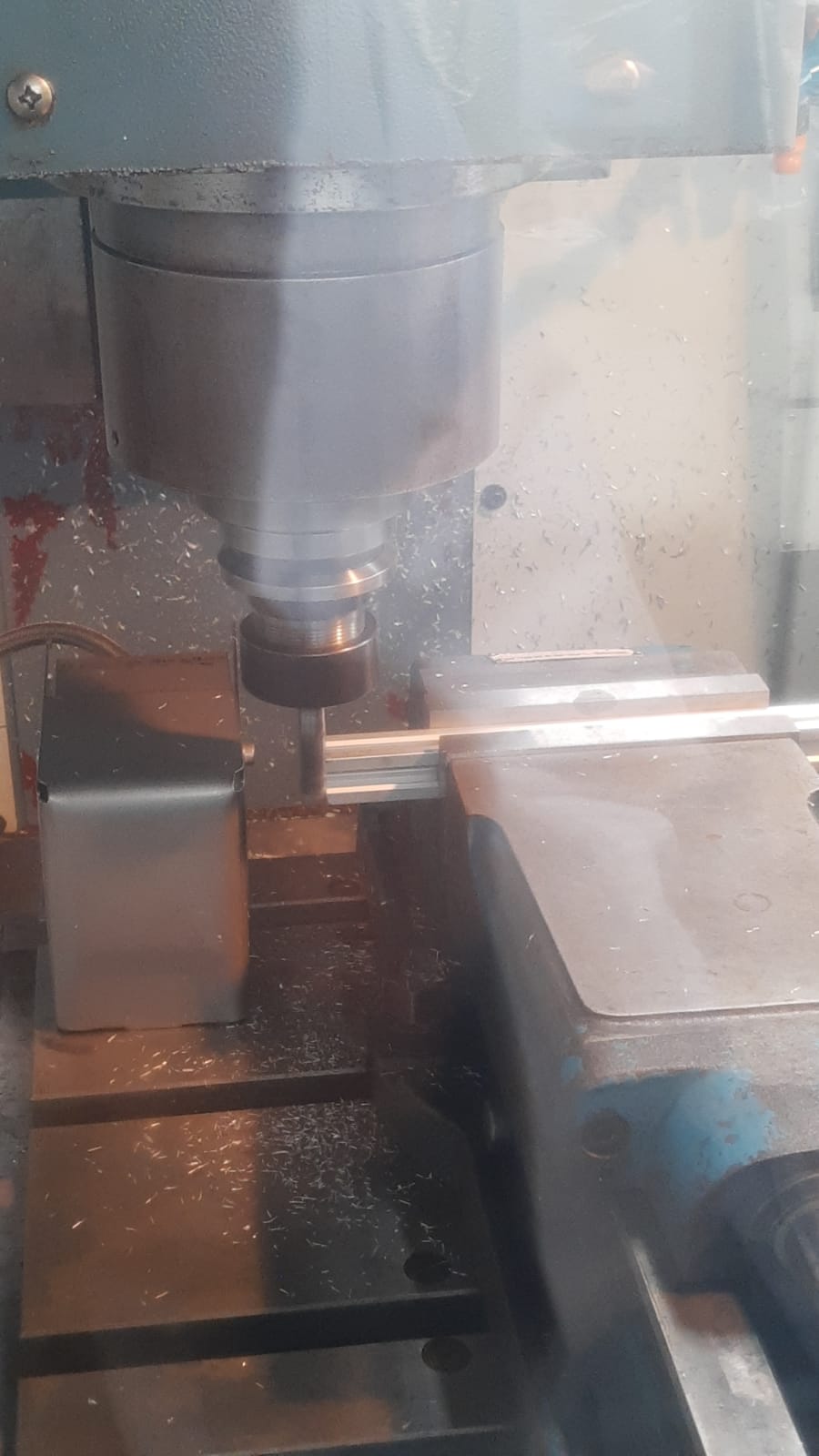
Milling of the aluminium profile.
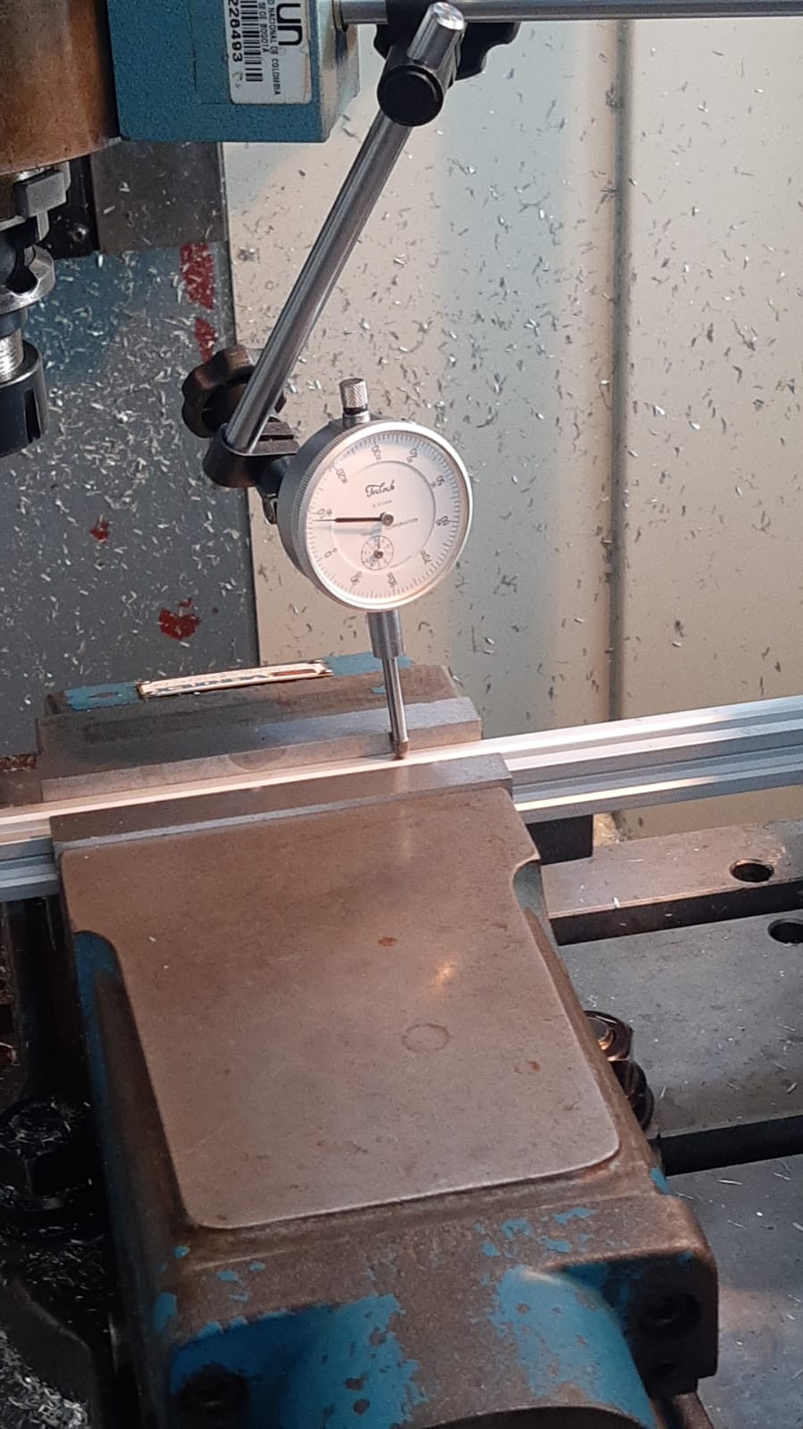
Profile cutting assembly
The axis rods were cut using an angle grinder, as the ends of it were free as no element blocked both ends. This was done by the LabFabEx technician as shown in figure manufactura10.
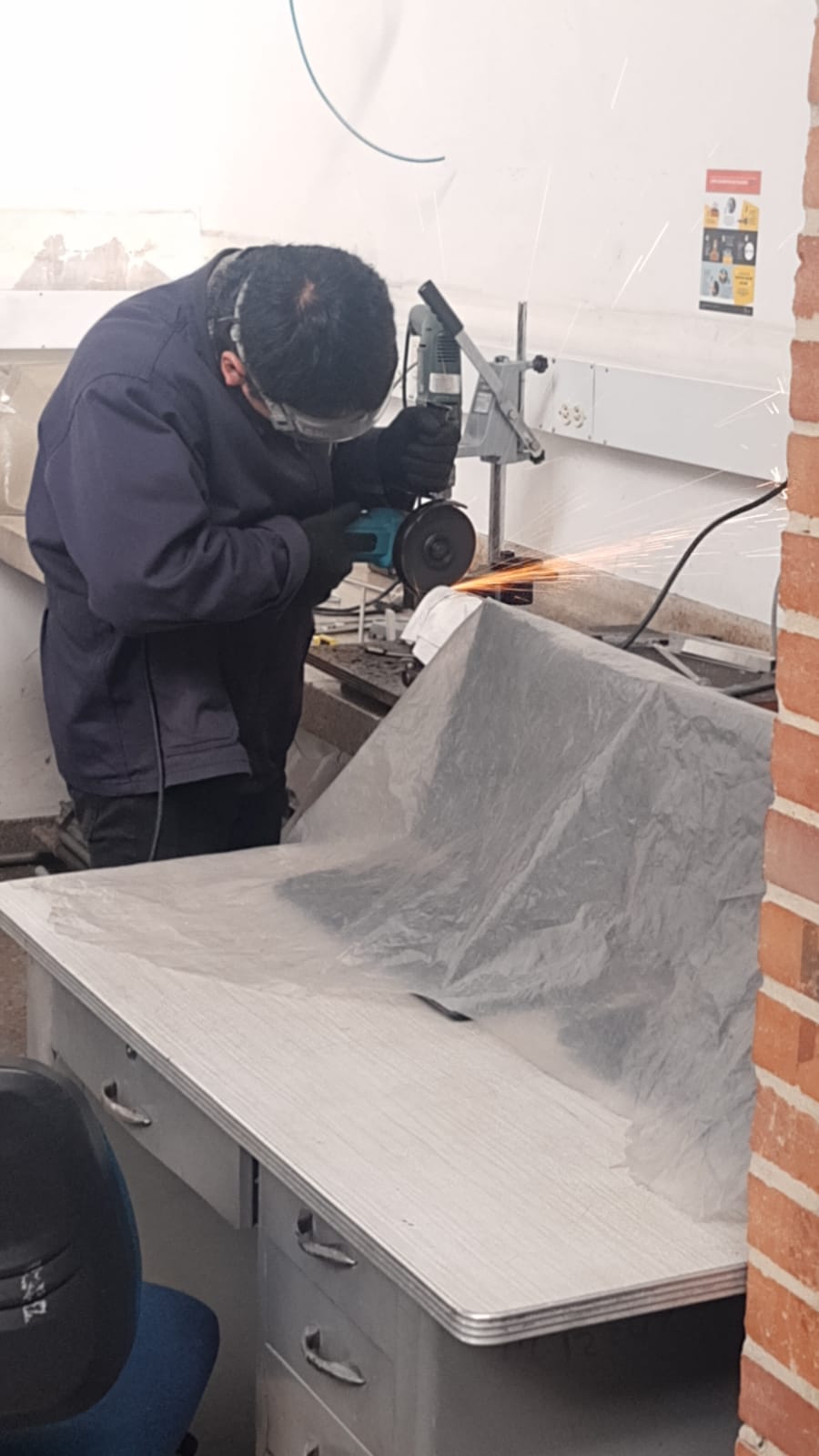
Axis rod cutting
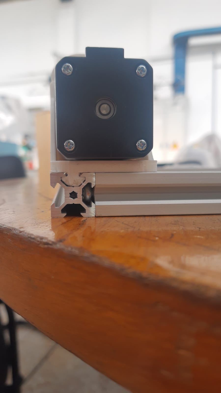
The corner assembly is shown in te next figure, where the motor support and two brackets are mounted, they were inspected on rigidity and no movement was found, proceeding with the next section assembly. For the X axis the supports are paired by left and right, each one containing a motor support and a leadscrew support. The last one counts with 628ZZ radial bearings to place the leadscrew.
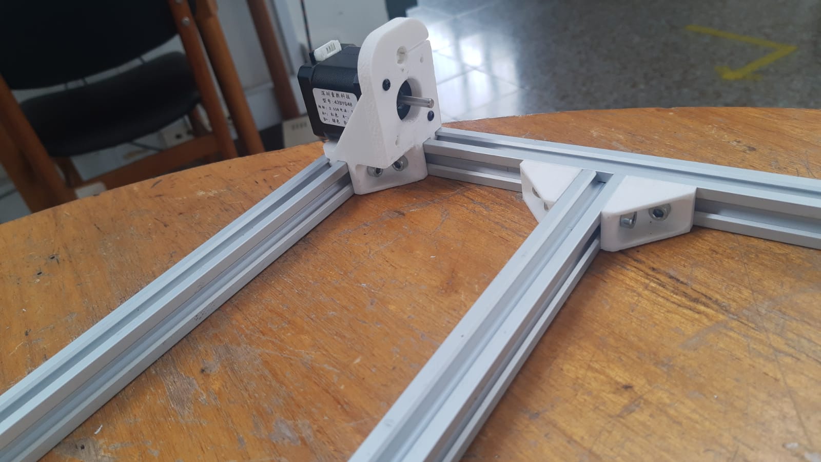
Assembly of the corner of the machine
Afterwards, the support for the other 2 axis carriages was assembled, each one has two LM800U linear bearings, that slide over the axial rods. Movement is transmitted over the leadscrew, using the bronze anti-backlash nut shown in figure manufactura4.
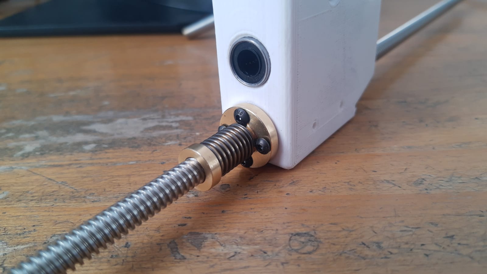
Leadscrew with the Y axis support
Motion
Three motion characteristics were analyzed, the capacity to generate a higher order motion profile, the maximum rapid motion and the critical angle velocity of the leadscrew.
- Smoothed Jerk Control: The objective of smoothing the control of trajectories is to convert the trapezoidal profile into an S-type profile. To achieve this, the following equipment was researched:
- SmoothieBoard V2: A 32-bit control board (compared to the 8-bit Arduino UNO), using the Smoothie software. The mini version of this board costs \(90\) Euros.
-
LinuxCNC: A control software that runs on Linux, but requires a x64 or x86 architecture machine. The user hydroid7 created a branch with a smoothed trajectory planner.
- Mach4:Through the SmoothStepper board, however, it uses separate drivers, so you have to buy a breakout board. This board costs \(226\) US Dollars.
In no case was it found that the microprocessor with which the PCB Mill is equipped does not support the movement of profiles of higher order than trapezoidal, so it would be necessary to modify the control equipment and the board that would have the drivers. Doing so would increase the cost of the machine significantly.
-
Critical Angular Velocity of the Power Screw: The objective of calculating the critical velocity of the screw is to avoid resonance, which can cause damage to the system. Resonance occurs when the natural frequency of the system coincides with the frequency of an external force, such as the force applied by the motor to the screw. When this happens, the system vibrates with great amplitude, which can damage the mechanical components.
The critical velocity of the screw can be calculated using the following formula:
\[N=\frac{Cd_r \cdot 10^7}{L^2}\]where:
- \(N\) is the critical velocity in \(rpm\)
- \(d_r\) is the minor diameter (root) of the power screw in $mm$
- \(L\) is the length between supporting bearings in $mm$
\(C\) is a coefficient based on the mounting of the brackets in figure coeficient

C coeficients by Thomson
The coefficient C depends on the type of mounting of the screw supports. The PCB Mill uses “C”-type supports, so the coefficient C is \(0.25\).
The complete range of coeficients are shown in table.
| C | End 1 | End 2 |
|---|---|---|
| 3.9 | Fixed | Free |
| 12.1 | Simple | Simple |
| 18.7 | Fixed | Simple |
| 27.2 | Fixed | Fixed |
C coeficients values
For the case of the PCB Mill, with a minor diameter of 12 mm and a length between bearings of 110 mm, the critical velocity is:
\[N = \frac{18.76 \cdot 6.1 \cdot 10^7}{50^2} = 4562800\, rpm\]Converted to angular velocity, the critical velocity is:
\[\omega = 2\pi N = 2\pi \cdot 4562800 = 238907.6 \,rad\]The critical angular velocity of the PCB Mill is 238907.6 rad. It is important to prevent the power screw from operating at this speed, as it could enter resonance and be damaged.
-
Maximum rapid motion
The capacity of GRBL to transmit data was analyzed. Based on the speed response estimation performed by grblHAL, a modification of GRBL to run on 32-bit devices (such as a Teensy 4.1 microcontroller for example), the following estimation was made.
Considering that the Nema 17 motors used have \(200\) steps per revolution, the power screw of the X axis has a feed of \(2\,mm\) per revolution, it is found that every \(100\) steps \(1\, mm\) will be traveled; likewise, the maximum working speed defined by the design is \(60 \frac{mm}{s}\), so that it would have to move \(6000\) steps per second, in other words the steps will work at a frequency of \(6kHz\), which is within the limit of \(30kHz\) offered by a controller such as the Atmega328p that the Arduino UNO has running GRBL.
On the other hand, the motors have a maximum speed of \(3000\,rpm\), and considering the feed of \(2\,mm\) per revolution, it is found that the maximum feed speed would be \(100\frac{mm}{s}\), based on the criteria of the motors.
Vibration Analysis
Multiple methods to analyze the structure natural frequency was used, with different results according to the modelling used.
Taking into consideration the model proposed by Kopets for the following equation:
\[f=\frac{1}{2 \pi} \sqrt{\frac{\sum_i k_i}{\sum_i J_i}}\] \[\frac{1}{2 \pi} \sqrt{\frac{4k_1+4k_1+2k_2}{4M_{v1} L_1^{2} + 2M_{v2} L_3^{2}+M_{H} L_1^{2}+3M_{m} L_1^{2} + M_m (L_1 + L_3)^2 + 2M_{G1}L_1^2 + M_{G2} (L_1 + L_3)^2 + \frac{2 M_{G3} (L_1 + L_3)^2}{3} }}\]| Parameter | Value |
|---|---|
| Torsional Stifness of printed piece \(k_1\) | \(1.3572e+04\) |
| Torsional stifness of dremel carriage \(k_2\) | \(1.7379e+04\) |
| Printed support mass \(M_{v1}\) | \(0.059\) |
| Y carriage printed support mass \(M_{v2}\) | \(0.103\) |
| Machine head mass \(M_H\) | \(0.9850\) |
| Motors mass \(M_M\) | \(0.2850\) |
| X axis rod mass \(M_{G1}\) | \(0.2080\) |
| Y axis rod mass \(M_{G2}\) | \(0.12\) |
| Z axis rod mass \(M_{G3}\) | \(0.0548\) |
| Base lenght \(L_1\) | \(0.07\) |
| Carriage lenght \(L_3\) | \(0.071\) |
Frequency Estimation using Kopets
Obtaning that \(f=352.79 \, Hz\).
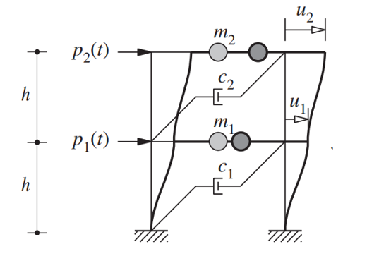
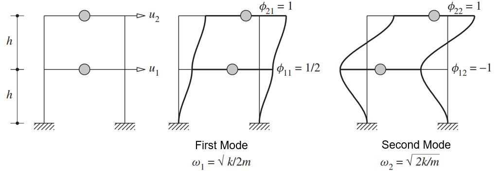
Using Chopra method to analyze structures based on multilevel structures, for this case, due to the axial rod and power screw for the x-axis on each end of the y axis (shown in figure vibration1), a two story model was selected.

Structure subassembly used for the analisis
This model has the following characteristics:
- 2 Degree of freedom system
- No damping support
- First and second vibration mode
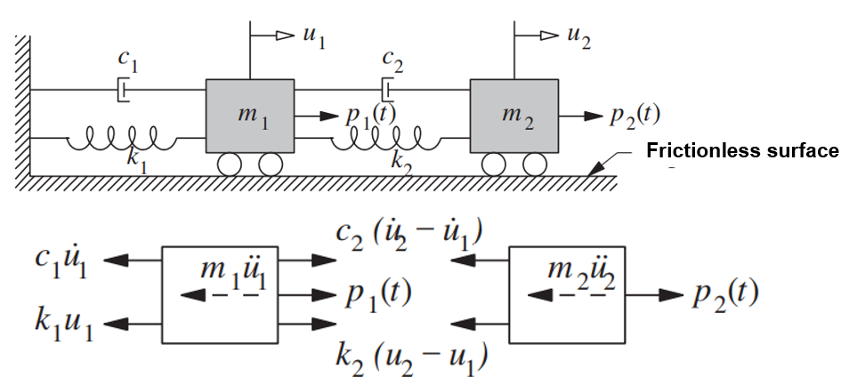
The model counts with three types of representation methods the first corresponds to a two level, mass centered structure (vibration2).
Structure model used
The second model is a dynamic model of a mass cart on a friction-less surface, and third the cart’s free body diagram, both are shown in figure vibration3. Take into account this representation shows damping, yet the PCB structure has a damping value of $0$.
Other representations of the system
According to Chopra, the deduction of the frequency vector is as follows:

The stifness of each level is obtained this way:
\[k_j = \sum_{columns} \frac{12 EI_c}{h^3}\] \[k_1=2 \frac{12(2EI_c)}{h^3} = \frac{48 EI_c}{h^3}\] \[k_2 = \frac{12(EI_c)}{h^3} = \frac{24 EI_c}{h^3}\]And the first two modes of vibration are:
\(det[k-\omega_n^{2} m]=0\) \((2m^2)\omega^4 + (-5km)\omega^2 + 2k^2\) \(w_1 = \sqrt{\frac{k}{2m}}\) \(w_2 = \sqrt{\frac{2k}{m}}\)
A diagram showing the physical representation is shown in figure vibration5.
FoS on the Angle bracket in its standard functioning
For the machine the values of the equation are:
\[I_c=2.53 \cdot10^{-6}\] \[E=2.5 \, GPa\] \[m=1.669\,kg\] \[T=\frac{2\pi}{\omega}\] \[f=\frac{1}{T}\]For the first vibration mode:
\[\omega_1 = 763.86 \, \frac{rad}{s}\] \[T_1=0.0082\,s\] \[f_1=121.57\,Hz\]And for the second mode:
\[\omega_2=915.35\, \frac{rad}{s}\] \[T_2=0.0069\,s\] \[f_2=145.68\,Hz\]Electronic Design
The machine is equipped with 4 Nema 17 1A motors, four DVR8825 Stepper motor drivers, a 12V, 10A source.
The connection diagram of the electronic components in this machine is observed in the next image.
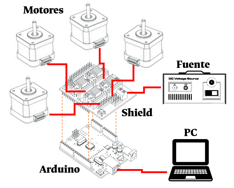
CNC connection diagram
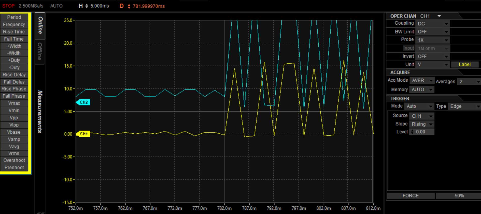
Initially, it was checked that the motion inputs on the DVR8825 drivers were synchronized, which corresponds to the synchronization of the Arduino outputs, which can be seen in the following two graphs. The first is the analysis of the difference between the Standby value and the pulse value (since it is a square wave).In figure desfasesubida the difference between both drivers is shown, with a closer look in the next figure.
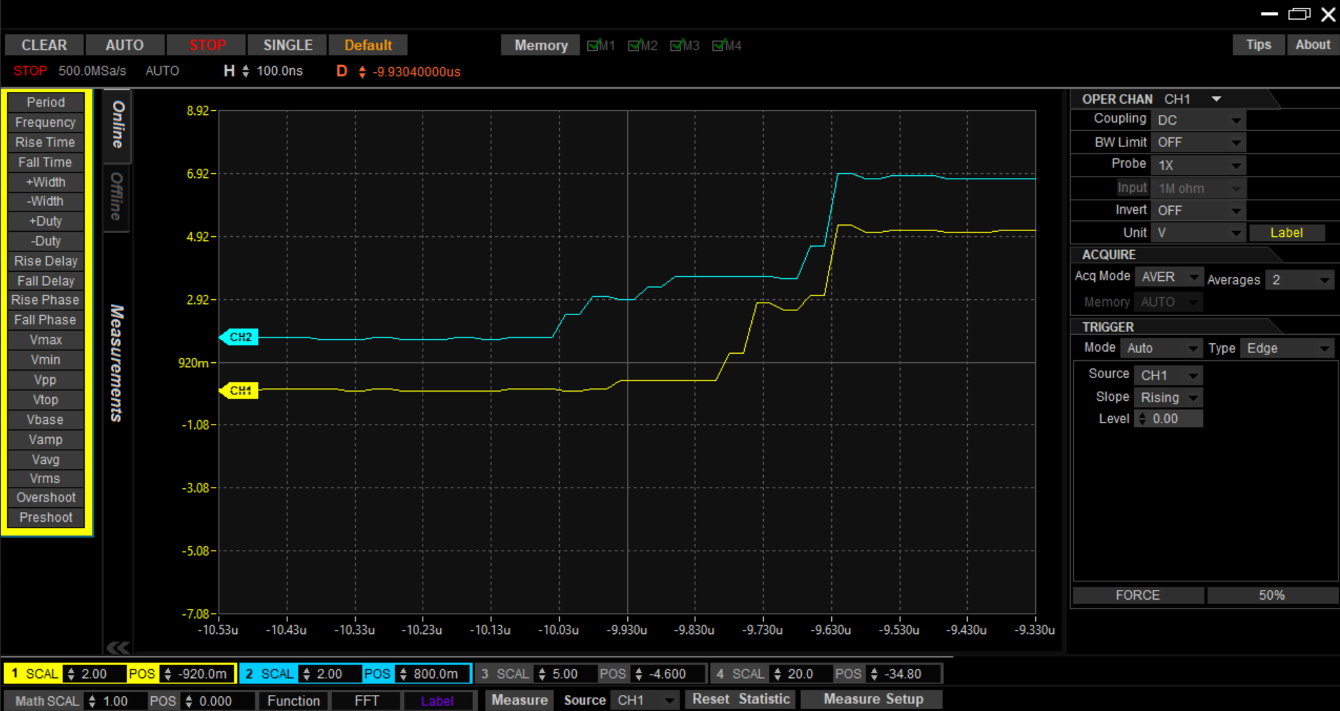
Driver activation signal offset
Upon expanding the measurement spectrum, it is identified that it is a signal whose phase shift is less than 5 ns, the measurement limit on the RIGOL DS 1074Z oscilloscope that was used.
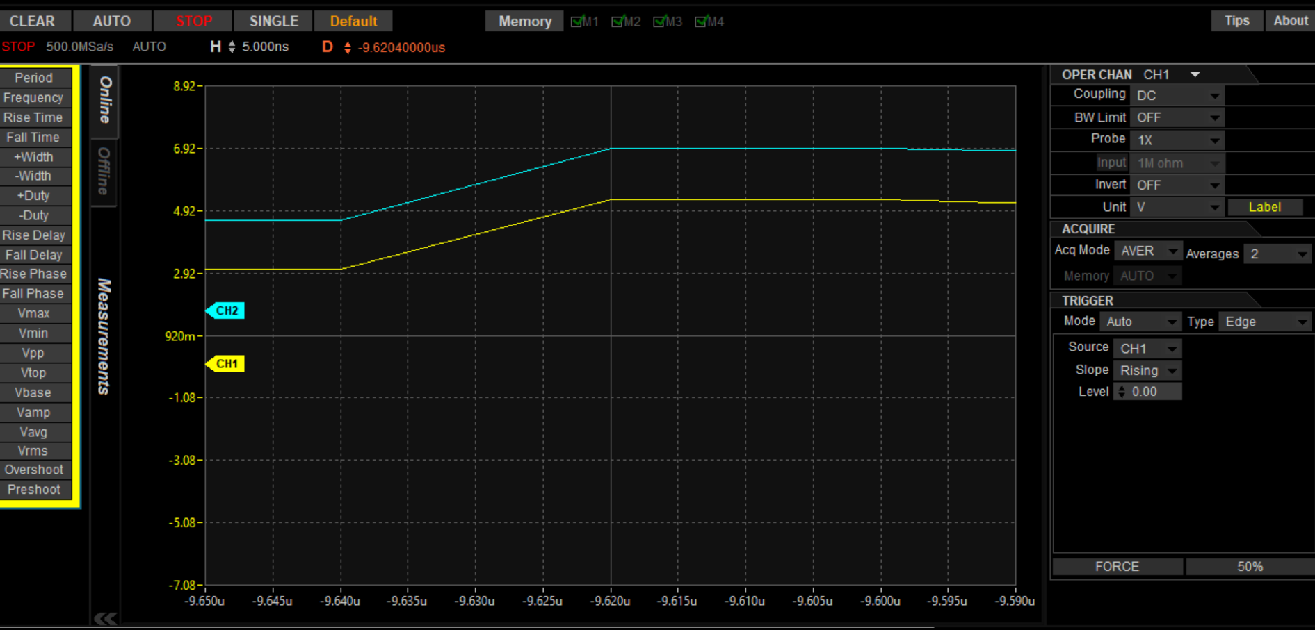
Detailed offset on drivers
Once it was verified that the reception time of the signal at the drivers did not have a large phase shift compared to the pulse time, the signal was verified in the coils of the motors. Specifically, the A2 coil of each of the motors on the X axis. Similarly to the previous one, the following graphs correspond to a visualization in two different time scales to have more detail about the phase shift.The coarse signal is shown in figure, and the finer one syncfino.
Motor signal offset
In this graph, a larger phase shift is found with respect to the input signal of the driver, however, since the signal is 12V, the oscilloscope does not allow visualization below 1us. In the image it can be observed that the phase shift is less than a quarter of the measurement step, so that although the difference is of the order of nanoseconds, the exact value cannot be determined with the equipment used.
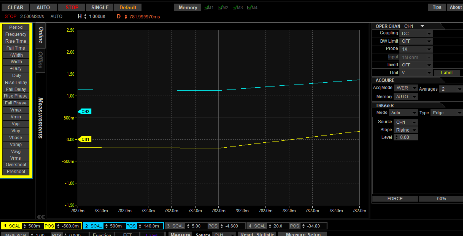
Motor signal offset in detail
File preparation
-
ECAD files: A normal gerber file must be loaded per face to mill, this microfactory was concieved using only one face of the PCW, therefore only one is needed. There are multiple Electronic Computer Aided Design (ECAD) tools like KiCAD, Proteus and Autodesk Fusion 360. Export the gerber files for the next step.
-
CAM files: Here the is where the Gcode files are produced, so there are multiple options to generate these files. Due to the application I recommend using FlatCAM, as it has automatic tools for PCB production, like automatic cutting depht calculation given a mill angle and type.
-
Gcode Sender: Files must be loaded into the Gcode sender software, they only recieve G code files, like
.gcodeor.ncfiles. There are two Gcode sender softwares being used in the moment, Universal Gcode Sender and CNCjs. CNCjs offers the capability of being installed in a debian device (like Raspberry Pi) to be used over a local network via UI at the device IP. Both have the capaciblity of controlling the machine position and reconfiguring GRBL parameters, likemm/revor maximum velocities.
First the maximum current allowed by the DRV8825 drivers is set by adjusting the potentiometer (with a philips screwdriver) voltage according to the following expression.
\[V_{ref} = \frac{I_{max}}{2}\]Afterward, the \(\frac{mm}{rev}\) units must be configured to verify the machine’s correct precision. For this the following equation was used:
\[\frac{motor \; steps \; per \; revolution}{leadscrew \; pitch \; (mm \; per \; rev)}\cdot microsteps\] \[= \frac{200}{8}\cdot 2 = 50\]And afterward, the advance per axis was configured with the code $ 100=50. This is done as well for 101 and 102.
The driver microsteps are configured trough jumpers in the CNC Shield. The pins in the connectors on M0, M1 and M2.
The machining process is currently using a \(60 \; \frac{mm}{s}\) feed rate, at a \(10000 \; rpm\) spindle speed and a cut depht of \(0.5\, mm\). It’s current precision is under a milimeter fraction.The machine is built using PLA printed parts with a \(60\%\) cubic pattern infill. It counts with 4 Nema 17 17HS4401S motors, with two parallel \(8 \; mm\) pitch power screws and A36 steel rods. It counts with a 10A 12V power source connected trough 16AWG gauge wire.
Currently the software usde is UGS, since the classic version offers a Command Line Interface (CLI) to execute tasks, specifically, it allows to run a Java command to mill a .gcode file. To do this, the device port must be allowed full access. Afterwards, the bin file in the Java folder is executed.
PRIA integration
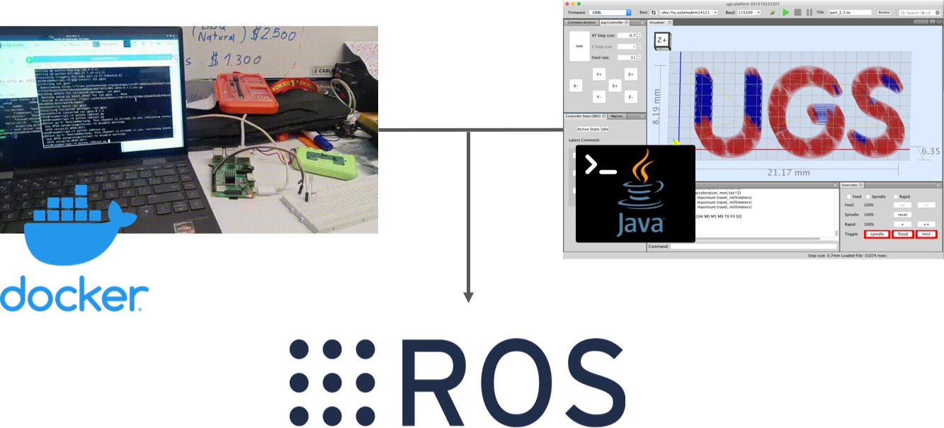
The deployment of the server is expected to be in either a Raspberry Pi device, or a Computer, as the host controller and Gcode sender software. Figure priacnc illustrates an example on a Raspberry Pi, with a Docker image containing the required packages to run the ROS nodes.
Completed Machine
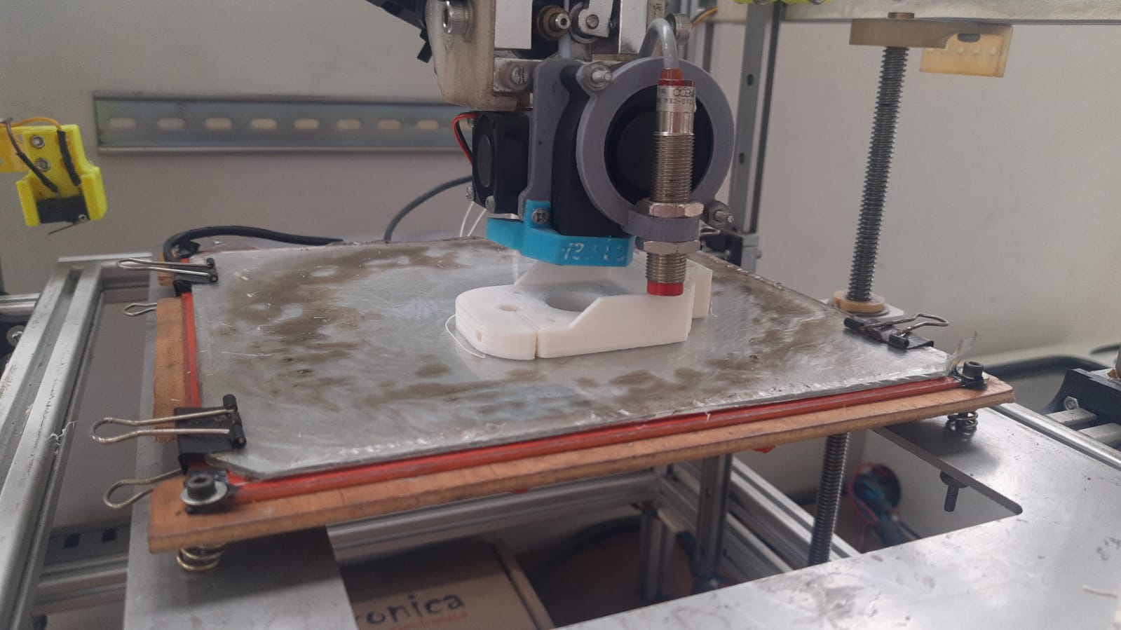
The PCB Mill is shown in the next image, with a pencil tool to draw figures, it is a removable accessory that fits in the Dremel holder.
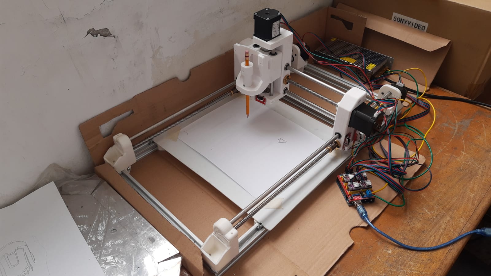
PCB Mill Completed Structure
In figure machinedpcb we see the result of a milled FR4 board using the machining parameters stated before.
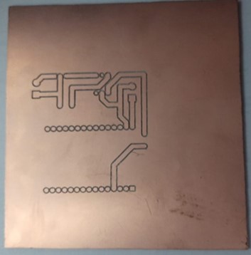
Milled PWB
Parameter Adjustment
First set the maximum current allowed by the DRV8825 drivers by adjusting the potentiometer (with a philips screwdriver) voltage according to the following expression.
\[V_{ref} = \frac{I_{max}}{2}\]Afterward, the $\frac{mm}{rev}$ units must be configured to verify the machine’s correct precision. For this, use the following equation:
\[\frac{motor \; steps \; per \; revolution}{leadscrew \; pitch \; (mm \; per \; rev)}\cdot microsteps\] \[= \frac{200}{8}\cdot 2 = 50\]And afterward configure the advance per axis with the code $100=50. Do this as well for 101 and 102.
The driver microsteps are configured trough jumpers in the CNC Shield. The pins in the connectors on M0, M1 and M2.